Improving our predictions of secular variation using estimates of flows of molten material in the Earth's core

Secular variation (SV) is typically defined as the slow annual to decadal change of the Earth's magnetic field and is caused by the flow of liquid in the outer core, deep inside the Earth. The change of the field is not easily predictable due to the nature of the flow regime in the core and the mechanism by which the magnetic field is generated. However, an estimate of the instantaneous flow itself can be computed, if we make some assumptions about its nature and how it affects the magnetic field we observe at the surface. If we have a longer series of data we can compute the accelerated flow too.

Researchers usually assume that the magnetic field is effectively ‘frozen’ into the liquid under the surface of the core-mantle boundary (CMB, approximately 3000 km below the Earth's surface). This means the magnetic field is advected by the flowing liquid (i.e. drifts along with it) over short timescales (< 10 years, say). In reality, the actual interaction between the liquid in the outer core and the magnetic field is far more complex and is currently poorly understood in detail. However, if the simplifying assumption is made that any observed change in the spatial pattern of the magnetic field is due to fluid flow, we can mathematically ‘invert’ the changes in the magnetic field we measure at and close to the surface of the planet to infer the pattern of fluid flow at the top of the outer core.

Using several years of magnetic field observations from observatories and satellites can help us build up a picture of what the large-scale flow patterns in the core look like (this is known as a 'steady flow model'). Figure 1 (top) shows an image of the changes of the magnetic field and the flow patterns that could cause this on the core-mantle boundary (continents shown for reference). In the Atlantic hemisphere, the flow tends to be relatively fast, while in the Pacific hemisphere it is slow or non-existent. The change of the magnetic field variation and hence the accelerated flow is about ten times smaller (bottom). This map also shows strong changes in the Indian Ocean, suggesting this is a location of relatively rapid acceleration.

Figure 1: [Left] Downward component (Z) of the global magnetic field SV and acceleration. [Right] Steady flow and acceleration models at the core-mantle boundary (continents shown for reference).

In a manner analogous to weather forecasting, we can imagine that this flow pattern 'pushes' (or advects) the magnetic field with it, should it continue to flow in this manner for several years. We can now use the flow and acceleration models to forecast the change in the magnetic field over a short period (2-5 years).

Improving the flow models by including magnetic diffusion

Magnetic fields can change by another process known as diffusion. This can be imagined as analogous to the manner in which a drop of ink diffuses in a glass of water. In this scenario, a concentration of magnetic field flux would slowly diffuse through a conductive material. In the Earth's core, the magnetic field diffuses slowly on large spatial scales but more quickly at smaller scales. Based on research in Metman et al. (2020), we included the effect of magnetic diffusion in the core as well as advection to test if this additional property would improve the forecast of the magnetic fields over a five year period.

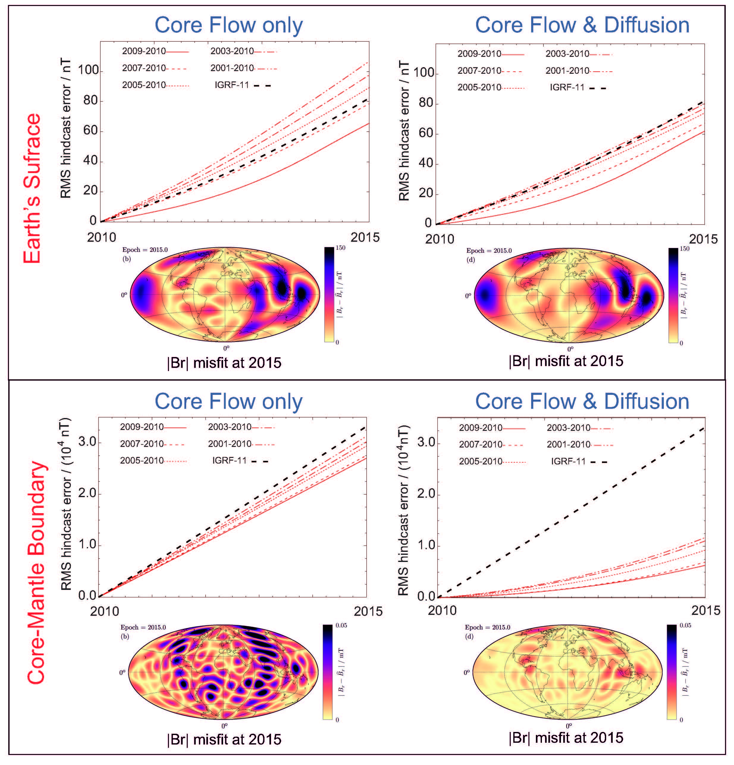
Figure 2 shows an example of how well flow models and diffusion can forecast magnetic change. Each line plot shows the root-mean-square (RMS) difference between a forecasting model and the 'true' magnetic field as measured between 2010 and 2015. The various lines with years labelled are different lengths of time used to invert for the flow or diffusion of the magnetic field prior to starting the forecast at 2010.0. In the upper panels, the forecasts from flow only and flow and diffusion are shown for the Earth's surface. The forecast model with the lowest RMS difference is when using flow and diffusion for 2009-2010 (i.e. one year). However, the difference between the left and right panels is very small, on the order less than 1 nT. The community-averaged model for the IGRF-11 is also shown. The best forecast would have improved upon it by around 15-20%. The images of the Earth show where the differences lie spatially at 2015 for the absolute value of the radial component of the field (|Br|).

The lower two panels show the RMS difference at the core-mantle boundary. In the left-hand line plot, the IGRF-11 forecast is now the poorest (note the scale has changed) while the 2009-2010 forecast is best. When the diffusion is added in, there is a significant improvement and the RMS difference reduces up to 75%. The images show where the differences are spatially on the CMB. Why is there such a strong improvement at the CMB but not the surface? The reason is that diffusion on timescales of five years mostly affects the smaller scales of the magnetic field. These are dominant on the core-mantle boundary but at the surface it is the large scales which are most influential on the secular variation. The upward continuation of the magnetic field from the core to the surface damps out the small scale features. Hence the upper right panels show only a minor improvement whereas the lower right panel shows a large improvement.

Figure 2: Comparing forecasts of secular variation from core flows only (left panels) with core flow and diffuson (right panels) at the Earth's surface (upper panels) and at the core-mantle boundary (lower panels).

The use of flow modelling to provide a more physics-based method improves the prediction of magnetic field change compared to simpler extrapolation methods. Further details can be found in Beggan and Whaler (2010), Beggan et al (2014) and Metman et al (2020). A review of the various forecasting methods for the IGRF-12 is given by Brown et al (2021).

References

 

Brown, W.J.; Beggan, C. D.; Cox, G. A. and Macmillan, S., 2021 The BGS candidate models for IGRF-13 with a retrospective analysis of IGRF-12 secular variation forecasts [in special issue: International Geomagnetic Reference Field - The Thirteenth Generation] Earth, Planets and Space, 73, 42. doi:10.1186/s40623-020-01301-3

Metman, Maurits C.; Beggan, C. D.; Livermore, P. W.; Mound, J. E., 2020 Forecasting yearly geomagnetic variation through sequential estimation of core flow and magnetic diffusion. Earth, Planets and Space, doi:10.1186/s40623-020-01193-3

Beggan, C. and Whaler, K. (2010), Forecasting secular variation using core flows, Earth Planets Space, 62 (10), 821-828, doi:10.5047/eps.2010.07.004

Beggan, C., Macmillan, S., Clarke, E., Hamilton, B. (2014). Improving models of the Earth's magnetic field for directional drilling applications. First Break, 32 (3). 53-60